Excel 2007- In Cell Dropdown List

When you need to enter data from a small subset of entries into a range in Excel 2007 you can do it more easily using a custom designed dropdown list.

To configure a dropdown list in a cell type the list of items to use in a single column in a spare sheet in the workbook.

Select these cells and choose the Formulas tab Define Name, type DataForList as the name in the dialog, set the scope to Workbook and click Ok.

Switch to the sheet where you want to add your dropdown list to some cells, select the cells that should display a list of data to choose from and choose Data tab > Data Validation > Settings tab.

From the Allow: dropdown list choose List and, in the Source area, type =DataForList and click Ok.

Now, whenever you click a cell in this range you’ll see a dropdown list appear from which you can choose a list entry for that cell.

If you're using Excel 2003, here is a link to an earlier post explaining how to do this in Excel 2003:

Automatic cell entries in Excel 2003
http://www.projectwoman.com/labels/validation.html

Excel 2007 - Check for Duplicates

The new Excel 2007 has far superior tools for finding and removing duplicate entries in a list. Thankfully - because this has been a nightmare in earlier versions.

To find and remove duplicates from a list of data in Excel 2007 first format the area as a table by selecting it and, from the Home tab, choose Format as Table.

Click on any cell in the table and choose Table Tools > Design tab on the Ribbon.

Select Remove Duplicates to display the Remove Duplicates dialog. In this dialog are the Column headings for your data and all are selected by default. To remove the duplicate data from your worksheet leave all the column headings selected and click Ok.

If you want to remove rows where only certain data matches, leave the column headings for those particular rows selected and deselect the column headings for those columns which may have data that differs from one row to another. Now click Ok.

It is sensible to save your worksheet before running this Remove Duplicates option just in case you delete data by accident. If this happens and if you haven't closed the file, you can recover it using the Undo button.


If you are using an earlier version of Excel, here are links to earlier relevant posts:
Excel - finding duplicates
http://www.projectwoman.com/2007/02/excel-finding-duplicates.html
Check for duplicates in an Excel list
http://www.projectwoman.com/2007/01/check-for-duplicates-in-excel-list-1.html

Excel macro – Format By Contents

You can do so much with Excel macros – they can be so powerful.

Here is a macro that formats a cell depending on its contents when you type something in it.

If you type a number, or a formula that returns a number, it is formatted one way, if you type a date it is formatted another way and if you type a word it is formatted a different way.

The macro uses the OnEntry event which fires whenever something is entered into a cell. If you attach the macro to an Auto_Open macro you'll ensure it is run whenever the workbook is opened.

To create the macro, choose Tools > Macro > Visual Basic Editor and, choose Insert > Module to add a module to the current worksheet. Type the code into the dialog.

Sub Auto_Open()
ActiveSheet.OnEntry = "formatCell"
End Sub

Sub formatCell()
If IsNumeric(ActiveCell) Then
ActiveCell.Font.Name = "Verdana"
ActiveCell.Font.Size = 12
ActiveCell.Font.ColorIndex = 46
ElseIf IsDate(ActiveCell) Then
ActiveCell.Font.Name = "Verdana"
ActiveCell.Font.Size = 10
ActiveCell.Font.ColorIndex = 50
Else
ActiveCell.Font.Name = "Times New Roman"
ActiveCell.Font.Size = 12
ActiveCell.Font.ColorIndex = 5
End If
End Sub

Sub Auto_Close()
ActiveSheet.OnEntry = ""
End Sub

Back in Excel choose Tools > Macro > Auto_Open to run the macro the first time to test it. Provided you have Excel configured to run macros, it will run automatically every time you open the workbook in future.

To learn more about Auto_open, AutoOpen and other fun macro naming conventions in VBA, visit this blog post:

What's in a name? Auto_Open or AutoOpen What's in a name? Auto_Open or AutoOpen
http://www.projectwoman.com/labels/Auto_Open.html

Excel: Print a worksheet your way

When you need to print one version of a worksheet for yourself and another for the boss and you like it small and he likes it to be - well just how he likes it, then you need Views. The Excel Views tool lets you configure a worksheet for different printing options and to save these so you can use them again later on.

You can set views up so you do one for your boss and one for you. Or, you can set one up to print only the summary part of a worksheet and another to print the lot. Even if the print areas and the print settings change, Views let you preconfigure them so you don’t have to set them up manually every time. Better still, Views are saved with the worksheet so they're always available.

Step 1
To save a set of printing settings, first set up your worksheet with the print settings you want to use including setting a print area if needed.

Step 2
To save this set up, choose View > Custom Views > Add (in Excel 2007 choose the View tab > Custom Views > Add). Type a name for the view that explains what settings you have selected. Enable the Print Settings checkbox and click Ok. You can now create another view and save it. Do this for as many different settings as you need. Save your worksheet.

Step 3
In future, before you print, choose View > Custom Views > select the View you want to use and click Show. Now go and print the worksheet - your settings were saved so you don't need to configure them.

Excel page headers and footers

When you're printing a 50 page worksheet, you want to hold onto the printed pages very carefully. If you don't the entire project is prone to disaster as it is all too easy for the pages to get out of order and it’s nearly impossible to sort out the mess. So, either staple them very quickly or use the header and footer tool in Excel to add page numbers to all your pages.

Of course, while page numbers are one of the most common things you might put in a header or footer it isn't the only thing. You can add everything from the date to your company’s logo.

To add a header or footer that will print on every page of an Excel workbook, choose View > Header and Footer in Excel 2003 or, in Excel 2007 choose Insert tab > Header & Footer. In Excel 2003 you can select from a range of preset headers and footers which are configured using typical combinations of items usually used in headers or footers – for example, sheet and worksheet names, page numbers, filename and folders.

If you'd prefer to create your own headers and footers, click the Custom Header or Custom Footer button and create your own design - this is the way you create a header or footer in Excel 2007 too.

Click in the Left, Center or Right areas of the dialog to place information at any of these places on the page. In Excel 2003 the buttons you can select from to add preset information aren't labelled but you can usually tell what they are. From left to right, they let you change the font used, insert the page number, number of pages, date, time, filename and folder, filename, sheet name, and an image. In Excel 2007 they are labelled.

When adding an image to a header or a footer, make sure it is small enough to fit in the header area – there's no tool in this dialog to resize the image if it's too big. When you're done, check the header by selecting Print Preview.

Multi colored Excel charts

It isn't always the case that you want to chart multiple series of data on a single chart. Sometimes you only have a single series and Excel, by default, plots all the bars or columns so they are colored identically. Boring!

Luckily, in Excel 2007 a solution is at hand. Simply select and right click the series and choose Format Data Series > Fill > Vary Colors by Point. Excel colors each bar a different color. Best of all, the colors are linked to themes so you can change the colors by changing the Theme - the theme tools are on the Page Layout tab.

So, no more boring single color charts - ever - please!

Excel - calculating workdays with Networkdays

Excel has lots of very cool functions for doing all sorts of calculations. One of these is the NETWORKDAYS function.

You can use it to calculate the number of days between two dates taking into account holidays.

Start by placing the dates for the holidays in a range of cells across a row or down a column. Select this range and name it holidays using Insert > Name > Define.

The function calculates the number of workdays between two dates so place one, for now, in cell A1 and the other in A2. This function will calculate the days between the dates in cells A1 and A2 taking into account the holidays listed in the range called Holidays:

=NETWORKDAYS(A1,A2,Holidays)

If the NETWORKDAYS function returns an error make sure that you have the Analysis Toolpak installed as this function is stored in this toolpak. To install it in Excel 2003 choose Tools > Add-ins and enable its checkbox. In Excel 2007, click the Microsoft Office Button > Excel Options > Add-Ins and from the Manage list choose Excel Add-ins and click Go. In the Add-Ins Available list enable the Analysis ToolPak checkbox and click OK.

Copy a worksheet - Excel 2007

I work with monthly worksheets and they develop over the month in such a way that I want the starting point for the next month to be where this month stops. So, I need to copy this month's worksheet to make next month's.

In Excel this is simple. Right click the tab at the foot of the worksheet and choose Move or Copy sheet. Make sure you click the Create a Copy checkbox so you make a copy or you're toast - you'll lose your original.

Now choose the position in the current workbook to make the copy or choose another or new workbook. Click OK and the copy is made.

I then strip out all of last month's variable data and start over for this month... but I always make sure I made a copy before I do this, you never can be too sure.

Excel 2007: quick format your data

I earlier versions of Excel there were some pretty horrid autoformats you could use to quickly format your tables. These are gone from Excel 2007 - thankfully!

Instead, Excel 2007 offers sophisticated formatting options, but they can be applied only if you're prepared to convert your range to a table. However, this isn't always a desirable outcome but luckily there is a work around.

Start by selecting your data and click Home tab > Format as Table and select a table format. You will notice that Excel applies an AutoFilter to your data which is typically the most obvious part of the conversion that you don't want. Other things come with this table format too - if you have data alongside the table – but not part of it - and you delete a row from a table or insert a row into a table, the data alongside remains in place.

So, if you want to retain the nice formatting but not the table behaviour, click in the table and choose Table Tools > Design tab and click the Convert to Range option and click Yes when prompted to convert the table to a normal range. The range will go back to behaving like a typical Excel range and the formatting will be retained.

Excel: Open multiple workbooks

If you're like me, you will open Excel in the morning and then open a series of workbooks that you work on each day. You can save time in finding and loading these files by creating an Excel Workspace.

To do this, open all the workbooks you want to have opened each time you launch Excel and then save them as a Workspace file by choosing File > Save Workspace and type a name for the file. Click Save and you can then open all the workbooks at one time by opening the Workspace file. Of course, if you just want to open a single file you can open it as normal.

In Excel 2007 - find the Workspace feature by choosing View > Window > Save Workspace.

Another alternative for opening files automatically when Excel opens is to save the file to the XLStart folder - when you do this, the file is opened every time Excel launches.

Fix the Headings in your Excel 2007 tables

Excel 2007 has some great tools for working with and formatting tables (previously called Lists in earlier versions). To create a table, select the range that contains the table data and from the Home tab select Format As Table. Select a table format style and, when prompted to, confirm that the selected area contains all the data for your table, whether or not your table has headers and click Ok. When you do this you will see that each heading cell displays a dropdown arrow to the right of its contents.

Unfortunately, if your headers are right aligned, the table headings will run into the arrows and be partially hidden. I don't know why Microsoft doesn't create a fix for this because it looks awful. To avoid this happening, select the heading cells, right click and choose Format Cells. Click the Custom setting and type @ and four spaces and click Ok. This should add sufficient spaces to the right of a heading to move the headings a little to the left so the headings can be seen clearly. Now it all looks much nicer as you see above.

Excel Change the Default font

If the default font that Excel 2003 uses for all new worksheets doesn't suit your needs - change it by selecting Tools > Options > General tab and set the Standard font and Size to your preferred choice and choose Ok.

In future, all new workbooks you create will be set by default to this font although those you have previously created will remain unchanged.

If you're using Excel 2007 and you don't fancy the new Calibri font, click the Office button, choose Excel Options and click the Popular group. From the Use this font dropdown list choose the font to use for your new worksheets and click Ok. You'll need to close Excel and restart it for the new font change to be in force.

Widening chart columns in Excel 2007

Colour me stupid. I am reeling from having single handedly wiped out all the images from my blogs - yep! 2 of them decimated by my stupidity. I'm now resorting to begging friends, family, neighbours and anyone I meet (ok I'm exaggerating, but I am desperate), to spend time helping me put it all back together. I have the images, they just aren't on my server any more and my computers and Blogger have this love hate relationship, the more frustrated I get with how slow the connection is the slower they go - see! they say, if you think that was slow, try this.. seriously it is hours of work to get this all back. Hence no delicious new posts.

This happened over two weeks ago so I'm slowly resigning myself to putting it back over time, so here's today's tip - no image - sheesh - don't talk to me about images!

To make the column widths on an Excel 2007 chart wider - or narrower if you think they aren't awful enough when you have long X-axis values, right click a column choose Format Data Series. From the Series Options selection drag the Gap Width value close to the No Gap end of the slider for a larger column and the other direction for a smaller one. This increases the column width by decreasing the gap between the columns. Click Close and you're done.

Now, back to uploading images one by one .. hell, even Noah got them in two by two!

Conditional formatting with Date ranges

One of the other handy features of the new conditional formatting tool in Excel 2007 is that it can handle date formatting. For example, if you have a worksheet with a series of dates in it you can highlight the dates that correspond to a period of time.

Choose Conditional Formatting > Highlight Cells Rules and choose the A Date Occurring option. You can then format cells using rules such as Yesterday, Today, in the last seven days, this month, next month, next week, etc.. When you do this cells containing dates which match this criteria will be coloured appropriately. Better still, when the date changes, the formatting on the worksheet will change accordingly.

Excel 2007 makes Lovely Lists

Lists were a big addition to Excel 2003 as they allowed you to work with list data in Excel more easily than ever before. One key plus was that they let you create charts that expanded automatically as the data in the list grew. This was something you simply couldn't do before very easily.

Now in Excel 2007 lists are called tables and they are simple to create using the Format As Table option on the Home tab on the Ribbon. One gotcha is that you shouldn't use a table format if you don't want to create a list, instead use the much more cumbersome and much less pretty Cell Styles options.

When you create a list you automatically get Filter buttons for the list. If you don't like or want them, disable them by clicking to disable the Filter button on the Data tab - just make sure your cell pointer is somewhere in the list when you do this. Like in Excel 2003, if you create a chart based on your table, it expands when you add new data to it.

Selecting chart elements in Excel 2007

It used to be easy to know what part of a chart you had selected in Excel 2003 - you just read the name off the left hand side of the Formula Bar.

Look in vain for this same feature in Excel 2007. Click anything on the chart and the formula bar just says Chart 1 - like duh! I know I have the chart selected it's the element on it that I'm interested in.

The solution is the new Chart Element tool. Click the chart to select it, choose Chart Tools > Format on the ribbon and in the top left corner is the Chart Element list. Not only will it tell you what you have selected on the chart but it's a dropdown list of names of various chart elements. Click one and that portion of the chart is selected automatically.

It's a handy new tool, I'd just like the benefits of the features from Excel 2003 and 2007 blended into one.. call me fussy.

Do You Undo?

This post is subtitled Undos that Do and Those that Don't

If you're using Excel 2003 or earlier, you have a big problem with the Undo command, you see much of the time, it plain doesn't work.

Curious? Try this: open an Excel file, make some changes to it (minor however, you won't be able to undo these however much you think you can). Check the Undo button - it is enabled. Save the file. Now check the Undo button again. Yikes, it's now disabled. You see, after you save a file in Excel 2003, all the Undo steps are removed - no more Undo. It pays to know this is how it works.

In Excel 2007, things are much better, and the Undo retains the changes even after you have saved the file. Much nicer behavior.

Excel charts - create an overlapping series

Sometimes an Excel chart will look better if your series overlap - this might be the case when you are comparing data from two years and where you want to show how the values have increased from one year to the next.

To make your series overlap in Excel 2007, select one series, right click and choose Format Data Series. Click the Series Options and decrease the Gap Width (it closes the chart up nicely) and incease the Series Overlap. Set the Series Overlap to around 60% and the Gap Width to around 30% for a good result. This is particularly useful when you are using images in place of colors for the bars of your chart but works in almost any situation.

In-cell charting in Excel 2007

For a long time Excel users have wanted a way to plot a bar showing the relative magnitude of a range of numbers without having to resort to a chart or complex formulas to do this.

Now, with Excel 2007 this feature is now built in and dead easy to use. To try it out, first type a series of numbers in a column, then select the series. Click the Home tab and click the Conditional Formatting button.

Select Data Bars and then select the color of the bar to use. The relative length of each colored bar indicates the relative value of the number in that cell.

There is one caution, however. All values - even very small values will be given a minimum bar length of 10% so they can be seen - so, use this feature as a guide and not an accurate measure.

Viewing Long Formulas - Excel 2007

If you've ever created a very long formula in Excel 2003 you'll know that it is difficult to see and to edit it - it simply is too big for the formula bar.

In Excel 2007 the problem is resolved, you can make the formula bar as big as you need it to be. Simply drag down on the bottom edge of the formula bar using your mouse, and it becomes as large as you need it to be.

Plotting little and big data

Disaster will strike your Excel charts if you try to plot very large data values and very small values on the one chart. You'll see the big values but the little ones will blend into the x-axis of the chart so you won't even see them.

To include both sets of data on the one chart, add a second axis and plot the smaller values against it. Now you'll be able to see them alongside the very large values.

To add your second axis, select the chart, select the series you can't see (click on one you can see and use the tab key to move until you have it selected). Right click and choose Format Data Series. Select Series Options, Secondary Y Axis. With the data series that should be plotted against the secondary axis still selected, right click and choose Change Series Chart Type and select a different chart type such as Line.

Error Checking in Excel

Chasing problems in Excel worksheets is a major pain. It helps to create them accurately in the first place but when you're trying after the fact, to find problems, Excel has some tools that can help. One of these is the often overlooked Go To option.

Go To can find formulas that vary from those in the cells that surround them. This can help you find formula errors which would otherwise be difficult to locate.

So, for example, if you have a column of cells which should all contain the same formula you can check to make sure they are written the same way by selecting the cells and choose Edit, Go To, Special, Column Differences (in Excel 2007, from the Home tab select Find & Select, Go To Special and then click Column Differences). Any cells which contain a formula that relates to a different series of cells to those in the active cell will be selected so you can check them. The Row Differences option does the same thing for rows of cells.

How-To with Helen Bradley

I write for lots of wonderful publications across the globe and one of them is Internet.com's Small Business Computing web site.

The great news is that I now have my own section and here it is: SmallBusinessComputing.com. Check a few sections down and you'll see a link to all my small business columns. There are heaps of columns on all things Office including Office 2007 and lots of stuff for earlier versions too. It's a great way to get down and dirty with some of the new features in Excel, PowerPoint and Word including Themes, SmartArt, Charts and lots of other handy tools.

Excel 2007 - Now where to?

When I enter data across a row in Excel it is extremely annoying when the cell pointer moves down instead of across when I press the Enter key. Luckily I know how to make it work for me and in a couple or four steps, it's doing what I want.

Click the Office Button, click Excel Options, Advanced and the first entry in the list is what you want. From the dropdown list select the movement option to use for the mouse and click Ok to end. Alternately disable the checkbox and the cell pointer won't move at all.

It's simple enough a process that you can change it whenever it suits you to do so.

Splitting data in Excel

Let's set the scene. You have a column in an Excel worksheet which contains a list of names, first name and last name all together. You want to split these into two columns, one for First name and one for last. How do you do this? Well one way is to use the Excel Text to Columns option.

Start by inserting a couple of columns to the right of the column which contains the names. Select the column containing the names and, in Excel 2007, click the Data tab on the Ribbon and choose Text to Columns. Step through the Wizard. In the first step choose Delimited and in Step 2 choose Space. Click Finish and answer Yes to the prompt to overwrite data. You will now have the data in two columns. You'll be able to remove the extra column you have there - it's best to add too many blank columns and later remove those you don't need because if you don't, you'll run the risk of losing the columns to the right of where you are working.

This is a simple and very fast solution for a name splitting problem.

Status bar functionality - Excel 2007

Right click the Status Bar in Excel 2007 and an entire grab bag of options open up for your choosing. You probably already knew that you could configure Excel in earlier versions to show you a single calculation on a selected range of cells - so you could select cells and then read the Sum of the values on the Status Bar (you did know that didn't you?) but the functionality is even better in Excel 2007.

Here you can choose to view an entire range of calculations so, instead of being forced to choose between Sum and Average you can have both display and throw in Min, Max and Count for good measure too!

You can also add a Macro Record button to use to fire off the Macro recording tool without having to delve into the ribbon to do so.

It all adds to your very slim customization pickings in Excel 2007 - make the most of it, this and the Quick Access toolbar are about all you've got to play with.

Don't look now! WordArt in Word 2007

If you've tried the new WordArt tool in PowerPoint 2007 you've probably discovered how neat it is. No more bent words in putrid magenta colors and instead, theme aware text that looks great for headings and which will change color when you change the Theme.

Try the same thing in Word 2007 and you're in for a ghastly surprise. WordArt missed out on getting a makeover in Word 2007 and, instead, it's the same application it has always been - functional but requiring a lot of additional work on behalf of the user to make it look even half good.

Here's hoping that the next implementation of Word, whenever that appears, finally does away with this and gives us WordArt that is usable and as functional as that in PowerPoint 2007 and Excel 2007.

Close everything NOW! Excel 2007 and PowerPoint 2007

Yum, it's like a boss key for Excel and PowerPoint. Double click the Office button in either application and it's like a Close All tool - everything closes quickly and automatically.

Doesn't work in Word, wonder why not?

Millions in Excel

Excel has some cool formatting tricks up its sleeve and one of these is its ability to shrink really big numbers down to size.

So, if you have values in the millions - like your salary - Ha!, you can size them down to size using a custom format. Select the cells, choose Format, Cells, Number tab and click the Custom group and type #,,"M" and Excel will format 200,000,000 to read 200M! The numbers aren't altered it's just a simpler way of displaying them.

Since the Y axis of a chart inherits its formatting from the top left cell in the chart data range this lets you format a chart's Y axis to show the smaller values too.

Changing Excel 2007 Default template location

Q: Where do you go to change the default locations for templates in Excel 2007?

Luckily I already know the answer to this question because my bet is that it’s going to take your hours to work out how to do it. You see, there’s no way in Excel to change the default location for where its templates are stored, in particular as one of my blog readers found to his chagrin, the default location for saving chart templates.

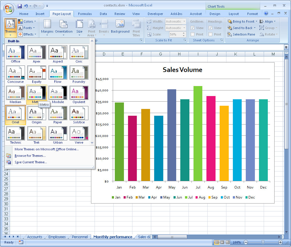
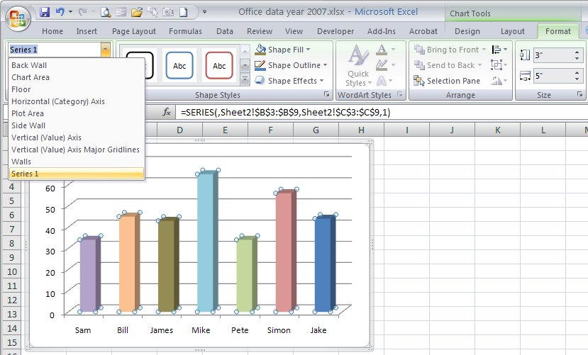
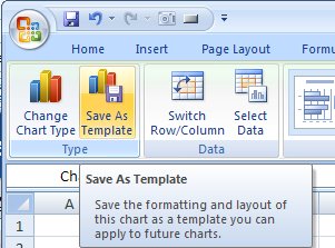
Perhaps I’ll start this story again, this time at the beginning. In a recent blog entry I showed you how to save a chart template. The process is this: create your chart in Excel 2007 and then from the Design tab which appears only when you have the chart selected, click the Save As Template button in the Type group and save your file in your default templates folder which should be c:\Documents and Settings\username\application data\Microsoft\templates. The file should have the .crtx extension.

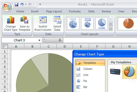
Close your Excel worksheet, close Excel, open Excel again, create the data for a new chart, select the data and choose Insert, Other Charts, All Chart types, Templates and your chart template should appear in the list. So far so good.

Problem is that not everyone’s installation of Excel 2007 looks to this default location for either saving chart templates or finding them when you need to use them. In particular you may confront this problem if you’re on a network. So the question then becomes where are your chart templates supposed to be saved to? Answer - who knows? You see, there's no setting in Excel to say where to put them, so you have no clue where Excel is looking for them, so you can't put them there because where is "there"?

So, we're now at the point where we know there’s no setting in Excel for specifying the default location for templates. If we could set this, we could save our template there and Excel could find it... simple to understand, but problematic to achieve.

The solution that I found and which works is to make the change in Word 2007 - not exactly the first place you'd look huh? If you visit this link: www.kbalertz.com/kb_924460.aspx you’ll see buried in the KnowledgeBase article quoted there, information on how the template locations in Office 2007 programs are managed.

There are some registry entries that you can change but the simpler solution is to change the location in which your templates are stored using the Word settings. When you use Word 2007 to change the location where your Word templates are stored you also change the location where all Office 2007 templates are stored. So Word’s settings control every other program which is sort of handy to know because you could spend all day looking in Excel for a place to change the Excel template location.

So here’s the short information on how to change Excel’s default template locations: --

Start Word 2007, click the Office button and choose Word Options, Advanced and locate the General group. Click File Locations, User Templates, Modify and in the modify location dialog change the setting in the folder name list or the look in list to point to the folder where your templates will be saved.

For ease of access and backup I suggest that you put it where they were supposed to be put in the first place which is Documents and Settings\username\Application Data\Microsoft\templates but theoretically you could put them anywhere.

This changes the setting in the Windows registry so that all templates are now saved to this location.

The KnowledgeBase article makes essential reading for anybody trying to manage Microsoft Office applications particularly in a network situation.

Quick moves in Excel

My friend Theda and I were talking the other day about a project she’s working on where she has to reorder a lot of items into alphabetical order and, in some cases, an order which is not alphabetical.

While she is doing the project in Microsoft Excel there are, of course, difficulties in Excel in moving items around as Excel does not, by default, open up a row when you choose to move an item from one part of the worksheet to another - instead, Excel thinks you want to overwrite the target cells - as if!

There is, however, a way to do this which opens up the space for the new row and which closes up the space that you have just made available. To do this select an entire row or range of rows in Excel by clicking on the row number or numbers. Hold your mouse over the dark outline around the rows and hold the Shift key as you drag the rows to their new position. The empty space that you have created will be closed up and a new space will be created between the other two rows for your item.

Problem solved!

Put a button on an Excel worksheet

I love the form tools in Excel they let you do so many cool things. One thing I love to do is to make buttons run my macros. To do this, use the Forms toolbar, click the Button tool and drag to create a button on the worksheet. When you do, a dialog appears with all your macros listed so you can select the one to use. You can also edit the text on the button and when you're done simply click it to run the macro - sweet huh?

If you're using Excel 2007 you have to add the button tool to your Quick Access toolbar (it's in the Commands Not In The Ribbon group and it's called Button (Form Control).

Camera Icon in Excel 2007

Hi Jim from Calgary!

Jim wrote and asked, "I’ve been using the camera icon for years and I can’t find it in Excel 2007. Can you see it anywhere?"

He also said, "nice blog thanks" - so anyone that nice deserves an answer.

So, Jim, don't go looking for the camera on the Ribbon it isn't there. You probably already know you can't customize the Ribbon either so you can't put it just anywhere you like - thanks Microsoft! You're limited to the Quick Access toolbar - that little bar to the right of the Office button. Click the down arrow to its immediate right and choose More Commands. From the Choose Commands From list choose 'Commands Not in the Ribbon' (that's how I figure it probably isn't on the ribbon), and then locate the Camera. Click it and click Add. Then click Ok. Now the camera is on the Quick Access Toolbar and it works as it always used to - least so far as I can see.

If you've now got a great new camera icon on your toolbar but you don't know what to do with it, then visit my Snap an Excel range blog entry to find out...

Reuse a Chart's "Look"

Sometimes you'll create a chart that just looks so good you want to save the 'look' so you can use it again. You can do this by turning your chart into a template. This would be a technique you could use if you were creating a report and you need to use multiple charts that are all formatted in a similar way.

To save a chart as a template, first display or create the chart and select it. On the Chart Tools, Design tab, choose Save As Template in the Type group. In the Save In box check you're using the Charts folder and type a name for your template and click Save. Later, to apply the template, to a chart you're about to create, select your data the Insert tab, click the Other Charts button to open the list and choose All Chart Types. Choose Templates and then the template you just saved. If you already have a chart created, click the chart and click the Design tab, then Change Chart Type. Click Templates, then click the template to use from the My Templates area.

You can store lots of templates to meet any need you might have and change from one to the other as required.

Too cool for school - Office 2007 SmartArt

New to Microsoft Office 2007 PowerPoint, Excel and Word is the SmartArt feature which is one you’re just going to love.

To test it out add a new slide to a PowerPoint presentation, for example, and select the blank layout. From the Insert tab on the Ribbon, select SmartArt and then one of the SmartArt objects.

I like the one called Staggered Process which I've shown here as it makes a great display for a simple step-by-step process. Select your choice of design and then you’ll see text brackets appear on the screen. Click in them or click the double-pointing arrows at the left of the SmartArt object and type your text in the special dialog.

Once you’ve got your bullet points in - and you can add more than the default three if you need more - you have a simple step-by-step graphic. But - this is only the beginning.

There are lots of different looks for your graphic including beveled edges and 3D effects, and you can choose these from the SmartArt styles dropdown list in front of you. You can also change the colors used in the design which, of course, are based on the current document Theme colors. Change the Design Ttheme and the look of the project changes with it.

It’s about as simple as it’s ever going to be to add great looking step-by-step graphics to a PowerPoint slide. They are, seriously, way cool...

Start Smart in Excel

When Excel starts a default new workbook displays. This workbook contains many of the default settings for Excel and it can be customized so it looks the way you want it to look.

You can configure the defaults for your starter Excel worksheet if you place your settings in one of the two Excel templates; Book.xlt and Sheet.xlt. Neither file is required but, if you have one or other, or both, stored in your XLStart folder then Excel opens them whenever it opens and uses the data you have stored in them as its own default settings.

When you're creating either or both of the files make sure to put the relevant settings in the right file. Book.xlt should contain the defaults for all new workbooks such as styles and toolbars.

Use Sheet.xlt for options appropriate for all new sheets in a workbook which are added when you choose Insert, Worksheet. A word of warning, when you save a workbook as sheet.xlt make sure it contains only one Sheet.

Excel 2007 goes total color!

It's always been confusing to me and my readers why you have an unlimited number of colors to choose from in Word but only a handful of really ugly colors to use in Excel. It doesn't make sense - do Word users have better design skills than Excel uses - do they think that those of us who create worksheets somehow won't be blindsided by how ugly the color combinations we're being served up are?

Well, if you've been hankering after a rich color palette for your worksheets, you need do so no more. Excel 2007 gives you access to a full range of 16 million colors from the colors dialog so that you can use these colors, for example, for formatting text, charts or drawn objects. You can also select a Theme which gives you instant access to colors that are selected from the same monochromatic group and guaranteed to look great together. The new and very colorful options in Excel 2007 are guaranteed to wow you!