Articles | Photoshop blog | Photography blog | about me | e-mail

Helen Bradley - MS Office Tips, Tricks and Tutorials

I'm a lifestyle journalist and I've been writing about office productivity software for a long time. Here you'll find handy hints, tips, tricks, techniques and tutorials on using software as diverse as Excel, Word, PowerPoint, Outlook, Access and Publisher from Microsoft and other applications that I love. My publishing credits include PC Magazine, Windows XP mag, CNet, PC User mag, SmallbusinessComputing.com, Winplanet and Sydney Morning Herald.

Thursday, July 30, 2009

Outlook 2007 - Find a Contact Address

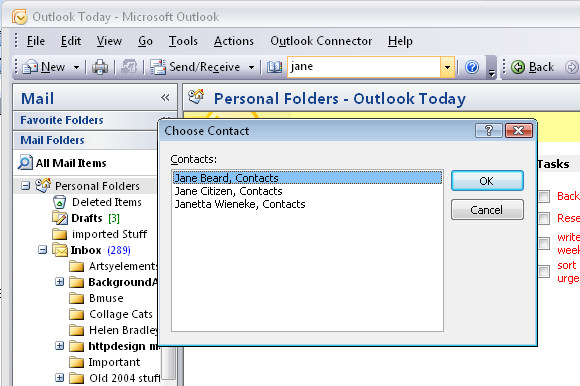
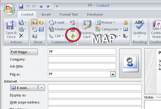
When you need to visit an Outlook contact and when you need directions to their office, you can find them yourself using Outlook's map option.

Select Contacts and open the contact's card. Click in the Address area so you are viewing the address that you want to find directions for. On the Ribbon, locate the Contact tab and in the Communicate group click the Map option. Your browser will open to display a map of the location you selected.

Labels: , , , ,

Add to Technorati Favorites

Wednesday, July 29, 2009

Excel macro – Format By Contents

You can do so much with Excel macros – they can be so powerful.

Here is a macro that formats a cell depending on its contents when you type something in it.

If you type a number, or a formula that returns a number, it is formatted one way, if you type a date it is formatted another way and if you type a word it is formatted a different way.

The macro uses the OnEntry event which fires whenever something is entered into a cell. If you attach the macro to an Auto_Open macro you'll ensure it is run whenever the workbook is opened.

To create the macro, choose Tools > Macro > Visual Basic Editor and, choose Insert > Module to add a module to the current worksheet. Type the code into the dialog.

Sub Auto_Open()
ActiveSheet.OnEntry = "formatCell"
End Sub

Sub formatCell()
If IsNumeric(ActiveCell) Then
ActiveCell.Font.Name = "Verdana"
ActiveCell.Font.Size = 12
ActiveCell.Font.ColorIndex = 46
ElseIf IsDate(ActiveCell) Then
ActiveCell.Font.Name = "Verdana"
ActiveCell.Font.Size = 10
ActiveCell.Font.ColorIndex = 50
Else
ActiveCell.Font.Name = "Times New Roman"
ActiveCell.Font.Size = 12
ActiveCell.Font.ColorIndex = 5
End If
End Sub

Sub Auto_Close()
ActiveSheet.OnEntry = ""
End Sub

Back in Excel choose Tools > Macro > Auto_Open to run the macro the first time to test it. Provided you have Excel configured to run macros, it will run automatically every time you open the workbook in future.

To learn more about Auto_open, AutoOpen and other fun macro naming conventions in VBA, visit this blog post:

What's in a name? Auto_Open or AutoOpen What's in a name? Auto_Open or AutoOpen
http://www.projectwoman.com/labels/Auto_Open.html

Labels: , , , , ,

Add to Technorati Favorites

Thursday, July 23, 2009

Excel: Monthly totals for daily data


One issue I was faced with recently was the need to calculate monthly totals for worksheet data that was recorded for every day of the month for a few years.

I had a long series of dates with corresponding data in the cells to the right which I had downloaded from the web. The data needed to be viewed as monthly totals rather than as daily values for me to have a better picture of the changes over time.

The solution to doing this quickly and easily is a PivotTable. Here’s how to do it:

1
Select all the daily data including the column headings. If you have lots more columns of data than you plan to analyze, don't worry, just select the lot for now.

2
In Excel 2007, choose Insert > Pivot Table. In the PivotTable Field List you now need to drag and drop fields into the respective boxes on the screen.

Drag the Date field into the Row Labels box and drag the field for the data that you want to analyze into the Sum Values box.

3
This gives you a list of dates and the data on the screen and you're over half way to your monthly totals.

Click on one of the dates in the Row Labels column to select that cell, right-click and choose Group to display the Grouping box.

4
Click both the Month and the Years values in the list so that both are highlighted. Then click Ok.

5
Now your data will reappear grouped by the year and by the month within that year.

This allows you to analyze how the data has changed over time more easily than viewing it by day.

6
From here, to chart your data, click somewhere in the PivotTable, choose Insert > and then from the Chart area on the Ribbon click the Column option to create a column charts.

Select the chart sub-type and you'll create a chart displaying the monthly totals from the PivotTable.

A PivotTable, while a little harder to get a feel for creating than a typical Excel formula, is actually the quickest and easiest way to summarizing this type data.

Labels: , , ,

Add to Technorati Favorites

Tuesday, July 21, 2009

Twitter - follow me follow you?


I'm often curious as to where I get some of my followers and I'd like to compare my followers with some other folk to see if I'm right in assuming I get some of my followers via them.

Enter this cool app called Followerlap. All you have to do is type two twitter ids, it doesn't have to be yours but it can be. So, if I want to see how many of my followers are also followers of, for example, Digital Photography School, I add:

HelenBradley and DigitalPS and click Submit.

Really it couldn't be easier. In a few seconds I know that nearly 20% of my followers also follow DigitalPS. Pretty neat hey?

Labels: , , , ,

Add to Technorati Favorites

Friday, July 17, 2009

Word 2007 - instant tables


New to Word 2007 is its Quick Tables feature which provides custom formatted tables for inserting in a document. To see the tables available click the Insert tab and choose Table > Quick Tables. The preconfigured tables include calendars and tables with sub headings and other features already formatted. Click a table to insert it and, once in the document replace the text in the table with your own text such as the dates for your desired calendar month.

These tables are a quick way to create some really great looking tables, one wonders though why no one made the calendar options just a little bit smarter so they automatically enter the desired month and days. Just a thought Microsoft!

Labels: , , ,

Add to Technorati Favorites

Thursday, July 16, 2009

Outlook 2007 Find a Contact Quickly

Wherever you happen to be in Outlook you can easily find a contact.

To do this, look to the Ribbon and locate the text box that contains the words "Search Address Books". Type part of the name in the box and press Enter.

This will locate all matching entries in the Outlook Contact list and display them in a dialog for you.

Choose the person to view and click Ok, their Contact details will then open allowing you to view their details, to email them or to send their details via email.

Labels: , , ,

Add to Technorati Favorites

Tuesday, July 14, 2009

Excel: Print a worksheet your way


When you need to print one version of a worksheet for yourself and another for the boss and you like it small and he likes it to be - well just how he likes it, then you need Views. The Excel Views tool lets you configure a worksheet for different printing options and to save these so you can use them again later on.

You can set views up so you do one for your boss and one for you. Or, you can set one up to print only the summary part of a worksheet and another to print the lot. Even if the print areas and the print settings change, Views let you preconfigure them so you don’t have to set them up manually every time. Better still, Views are saved with the worksheet so they're always available.

Step 1
To save a set of printing settings, first set up your worksheet with the print settings you want to use including setting a print area if needed.

Step 2
To save this set up, choose View > Custom Views > Add (in Excel 2007 choose the View tab > Custom Views > Add). Type a name for the view that explains what settings you have selected. Enable the Print Settings checkbox and click Ok. You can now create another view and save it. Do this for as many different settings as you need. Save your worksheet.

Step 3
In future, before you print, choose View > Custom Views > select the View you want to use and click Show. Now go and print the worksheet - your settings were saved so you don't need to configure them.

Labels: , , , ,

Add to Technorati Favorites

Thursday, July 9, 2009

Excel page headers and footers


When you're printing a 50 page worksheet, you want to hold onto the printed pages very carefully. If you don't the entire project is prone to disaster as it is all too easy for the pages to get out of order and it’s nearly impossible to sort out the mess. So, either staple them very quickly or use the header and footer tool in Excel to add page numbers to all your pages.

Of course, while page numbers are one of the most common things you might put in a header or footer it isn't the only thing. You can add everything from the date to your company’s logo.

To add a header or footer that will print on every page of an Excel workbook, choose View > Header and Footer in Excel 2003 or, in Excel 2007 choose Insert tab > Header & Footer. In Excel 2003 you can select from a range of preset headers and footers which are configured using typical combinations of items usually used in headers or footers – for example, sheet and worksheet names, page numbers, filename and folders.

If you'd prefer to create your own headers and footers, click the Custom Header or Custom Footer button and create your own design - this is the way you create a header or footer in Excel 2007 too.

Click in the Left, Center or Right areas of the dialog to place information at any of these places on the page. In Excel 2003 the buttons you can select from to add preset information aren't labelled but you can usually tell what they are. From left to right, they let you change the font used, insert the page number, number of pages, date, time, filename and folder, filename, sheet name, and an image. In Excel 2007 they are labelled.

When adding an image to a header or a footer, make sure it is small enough to fit in the header area – there's no tool in this dialog to resize the image if it's too big. When you're done, check the header by selecting Print Preview.

Labels: , , , ,

Add to Technorati Favorites

Wednesday, July 8, 2009

Word 2007 - Update Normal Style

The Normal style is applied to text by default if no other style is applied.

If the Normal style for any of the style sets is not to your liking, select it in the style list, right click and choose Modify.

You can now alter the style, for example you can reduce the inter-paragraph spacing by clicking Format > Paragraph and reduce the Spacing After value.

Click Ok and then, to apply this change to all new documents based on this template, select the New Documents Based on This Template option and click Ok.

By configuring the styles to suit your needs you can quickly format your documents to a consistent look without having to make all the format changes individually.

Labels: , , ,

Add to Technorati Favorites

Sunday, July 5, 2009

Protect an Excel worksheet


When you create a worksheet for others to use the last thing you want is for them to clobber your formulas or mess up your design. To keep them from making changes to the worksheet, either maliciously or inadvertantly, protect the worksheet.

If you haven't protected a workbook before you may find the process of doing so a little confusing. First you hage to unlock the cells that you want your user to have access to. These will be the cells that they can make changes to such as cells they need to add data to. You do this because all cells, by default, are locked against changes.

Select the cells the user should be able to change and choose Format > Cells > Protection and disable the locked checkbox.

Now choose Tools > Protection > Protect Sheet and, if desired, enter a password that will be required to unprotect the sheet so that it cannot be unprotected without permission. Click Ok and the cells that are locked — in other words everything that you didn’t unlock — will now be protected so that the user cannot change them.

The only cells your user will have access to are those that you unlocked for them to use. In this way, you can protect your formulas so that users cannot change them or overwrite them with fixed values which would render the worksheet potentially inaccurate.

Labels: , , ,

Add to Technorati Favorites

Friday, July 3, 2009

Social marketing with Twitter - find people to follow


When you’re developing a social marketing campaign using Twitter you will want to find people to follow who are the kind of people that you want to sell your services to.

Twitter’s advanced search tool at http://search.twitter.com/advanced can help you here. In the Advanced Search tool you can find Tweets based on words that are in the tweet or which contain a certain hashtag. You can find tweets by references to people or places as well as attitude or those that contain links.

Using this you can locate people within a specific geographical location or who appear to have an interest in something that you are interested in. By being able to find these people very quickly you can then follow them in the hopes that they will follow you back and so you build your follower list.

If, in time, you find that you have a lot of people who you are following and if you suspect that not all are following you, it is time to cull your following list. Visit this post to learn more about how to quickly cull your Twitter list as a batch job so you don’t have to do it one person at a time.

Labels: , ,

Add to Technorati Favorites

Wednesday, July 1, 2009

PowerPoint: Custom slide navigation with Action buttons


While many people make their presentations in the presence of an audience and they move from one slide to the next, not all presentations are delivered this way. Many slide shows are viewed by people at their desk and when you are creating presentations for display this way, you can create a custom navigation scheme for the user to use to progress through the show.

To do this, start by choosing View > Master > Slide Master to move to the Slide Master view. In PowerPoint 2007 select the topmost slide in the layout pane. Choose Slideshow > Action buttons and select the Action Button: Back or Previous. Click and drag the Action button on the slide – the Action Settings dialog shows Hyperlink To: Previous Slide - click Ok.

Repeat and this time add the Action Button: Forward or Next. This Action button is hyperlinked by default to the next slide.

Add an Action button that goes to the first slide by choosing Slideshow > Action buttons > Action Button: Home.

To size the Action buttons Control + Click on each of them in turn, right click and choose Format AutoShapes. Select the Size tab and adjust the width and height for all at the one time.

Click the Draw button on the Drawing toolbar, choose Align or Distribute > Distribute Horizontally to create even spacing between each button. Drag the shapes into the footer area so they are clear of the area covered by the slide content. Click Close Master View to return to your presentation.

Any shape can be configured to perform like an Action button. Add the shape to the slide, right click and choose Action Settings from the menu. You can hyperlink the shape to any slide, Office document or web page.

Labels: , , , ,

Add to Technorati Favorites