Excel: Charts that change

Create cool charts that you can change with a click of a button...

toper

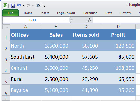
When you’re viewing complex data in Excel, it can help to see it more clearly if you limit what you see on the screen to what you are actually interested in seeing.

In this article I’ll explore an Excel solution that displays one of three charts and the associated data on the screen according to an option you choose from a dropdown list. The solution uses some handy Excel tools and it is driven by a simple Visual Basic macro.

Create the charts

To get started, enter some data into a range covered by A1 to D6 in your worksheet. I used data for a series of offices: North, South East, Central, Rural and Bayside in Column A and then provided information on the Sales, Items Sold and Profit in columns B, C and D. Column A and Row 1 are used to store the headings and the data is in the range B2:D6.

Step1

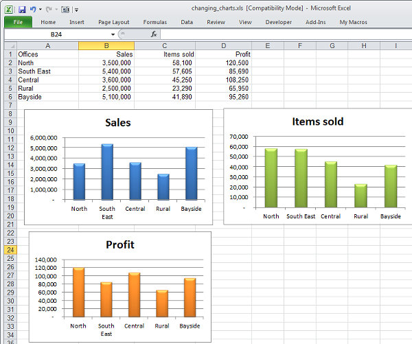
To create the charts, you will want one for each set of data. Select A1:B6 to and create a chart based on the data for Sales. Then select A1:A6, hold the Ctrl key and select C1:C6 and create a chart for the Items Sold. Finally, select A1:A6, hold the Ctrl key and select D1:D6 and create a final chart to show the Profit. For now, you can place these charts on the same worksheet as the data. Format the charts neatly.

Step 2

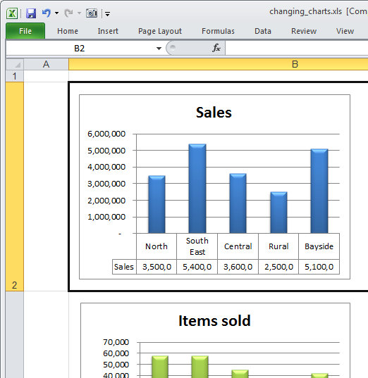
To add the relevant data to each chart, select each chart in turn, right click and choose Chart Tools > Layout > Data Table and choose Show Data Table. Only add a Data Table if it is an option for that chart type - it isn't an option for a Pie chart, for example.

Create the display sheet
To create the worksheet to display the data, switch to a new sheet and leaving row 1 empty, select row 2 and drag on the bottom border to enlarge the row. Drag on the right edge of column B to make the column much wider. You need to make cell B2 big enough to put one of your charts into it. Repeat and make Cells B3 and B4 just as big.

Return to your data sheet, select the chart for Sales, right-click it and choose Cut. Return to the display worksheet and paste the chart into cell B2. Repeat the process and add the Items Sold chart into cell B3 and the Profit chart into cell B4.

Step 4

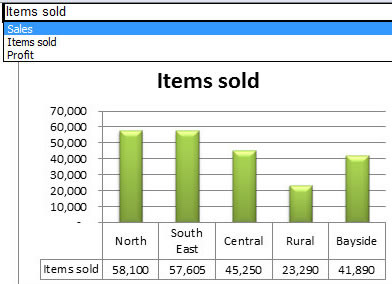
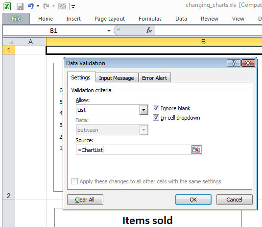
Add the dropdown list
Select the sheet containing your data and select the headings Sales, Items Sold and Profit (range B1:D1) and choose Formulat > Define Name, type ChartList as the name and click Ok.

Return to the display worksheet and click in cell B1 to create the dropdown list here. Choose Data > Data Validation > Data Validation > Settings tab. From the Allow dropdown list, choose List, make sure the In-cell dropdown checkbox is enabled and click in the Source area and type =ChartList and click Ok. This displays a dropdown list in the cell B1 which will show the three entries: Sales, Items Sold and Profit.

Step 5

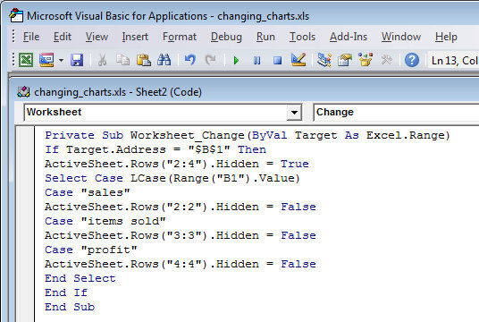
Now the basic display worksheet is complete you can format it by choosing View tab and disable the Gridlines and Headers checkboxes. This neatens up the display.

Add the code
To create the macro code that does the work of displaying the charts, select the sheet containing the charts, right click its sheet tab and choose View Code. This takes you to a special code sheet that includes events limited to the current sheet.

Into this code dialog, type this code and then choose File > Close and Return to Microsoft Excel:

Private Sub Worksheet_Change(ByVal Target As Excel.Range)
If Target.Address = "$B$1" Then
ActiveSheet.Rows("2:4").Hidden = True
Select Case LCase(Range("B1").Value)
Case "sales"
ActiveSheet.Rows("2:2").Hidden = False
Case "items sold"
ActiveSheet.Rows("3:3").Hidden = False
Case "profit"
ActiveSheet.Rows("4:4").Hidden = False
End Select
End If
End Sub

Step 6

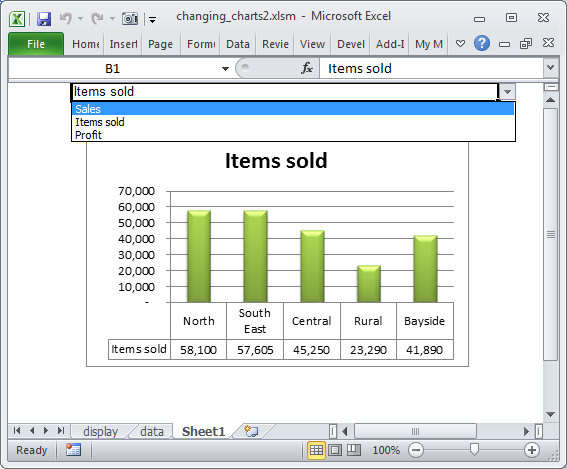
To test the macro, click the dropdown list in cell B1 and as you select an item from it, the worksheet should change to display the appropriate chart for that data. If it doesn't, make sure you have used the same names for the column headings as you used in the macro.

Step 7

How it works
This macro uses the Worksheet_Change event so that any change in any cell in the worksheet will trigger the macro to run. The macro tests to see if the change occurred in cell B1 and if it did not, then nothing happens. If the change was in cell B1, then rows 2, 3 and 4 of the worksheet are all hidden - this hides all the charts.

The macro then checks to see if the value in cell B1 is Sales. If so, it displays row 2. If it is Items Sold, it displays row 3, and if it is Profit, it displays row 4. Any time a cell in the worksheet changes, the macro will run and check cell B1 and update the display.