Wednesday, January 30th, 2008

Outlook: Managing Blocked Senders

I’m sure you’ve had that “that was a dumb thing to do” feeling before. You do something that you thought was smart but ends up being very silly indeed.

I got that recently when I added someone to my Outlook Blocked senders list. Yikes! they were so not supposed to go there!

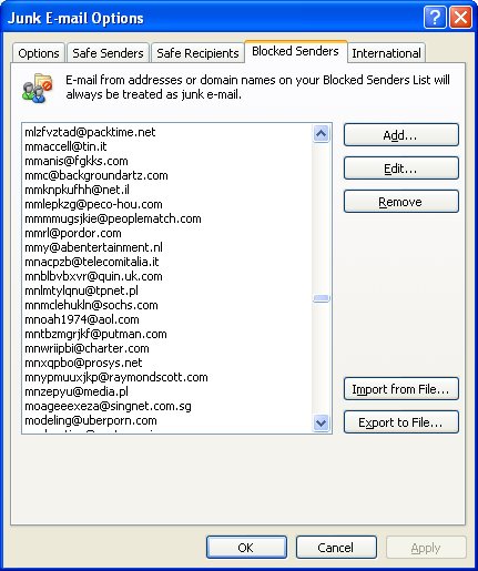
Luckily it’s fairly easy to undo the damage. In Outlook choose Tools > Options > Preferences tab and under the E-mail options click Junk E-mail. Click the Blocked Senders tab and locate the email address that shouldn’t be there and click Remove. Simple!

Now, if you need to go in reverse and add someone, here’s how (believe me, I’m astonishingly good at this step): In Outlook choose Tools > Options > Preferences tab and under the E-mail options click Junk E-mail. Click the Blocked Senders tab. This time click Add, type the email address or an entire domain name (but be sure you really want to do this!) and click Ok.

If you have an email from the person in your inbox there is an even easier solution. Right click the email, choose Junk E-mail > Add Sender to Blocked Senders List.

There you have it.. get someone onto the Blocked senders list and get them off again. Better still, it works in Outlook 2002, Outlook 2003 and Outlook 2007.

Helen Bradley

Saturday, January 26th, 2008

Excel 2007 makes Lovely Lists

Lists were a big addition to Excel 2003 as they allowed you to work with list data in Excel more easily than ever before. One key plus was that they let you create charts that expanded automatically as the data in the list grew. This was something you simply couldn’t do before very easily.

Now in Excel 2007 lists are called tables and they are simple to create using the Format As Table option on the Home tab on the Ribbon. One gotcha is that you shouldn’t use a table format if you don’t want to create a list, instead use the much more cumbersome and much less pretty Cell Styles options.

When you create a list you automatically get Filter buttons for the list. If you don’t like or want them, disable them by clicking to disable the Filter button on the Data tab – just make sure your cell pointer is somewhere in the list when you do this. Like in Excel 2003, if you create a chart based on your table, it expands when you add new data to it.

Helen Bradley

Thursday, January 24th, 2008

Cheung Chau Island, Hong Kong

When I was in Hong Kong I went first to order chops at Man Wa Lane (Chop Alley) which is in the Sheung Wan area of Hong Kong. Chops are stamps with your name engraved on them in Chinese characters that you use to sign things. Because they are your name and your birth year symbol, they ideally are hand carved for you. I have wanted one for years and there’s no better place to get it than Chop Alley.

With a few hours to spare until I had to pick up the chops, I headed by ferry to the wonderful Cheung Chau island. There are no cars here – everyone bikes or walks and it’s just the most wonderful place. One side of the island is a fishing port and the other side is beach.

This photo is from the fishing port side. The atmosphere was horribly grey and polluted so the image was totally lacking in color as well as having a pretty ghastly color cast. First step is to remove the color cast. I use the “color by the numbers” approach of sampling white, neutral and black areas of the image and then adjusting curves until they are within the ball park of correct. Then, I took the image to LAB to boost the color using curves on the A and B channels. You can’t do so easily unless you remove the color cast first. The result is wonderful and one of a series of boat images I’m working on.

Helen Bradley

Sunday, January 20th, 2008

Hong Kong Island tram

I’m not sure exactly what to say about this photo, it still takes my breath away every time I see it. It is so quintessentially Hong Kong.

Years ago they talked about taking out the trams, thankfully, reason prevailed and they didn’t. They are so unique and, in this photo, the tall tram, tall buildings and narrow roadway all work to give a wonderful perspective on this beautiful place.

Interestingly, the image can be cropped across the middle to give an equally beautiful and powerful image but, when it came to the crunch, I chose not to crop it. It’s this version that speaks to me, it’s what I saw and how I captured the scene, so here it is. Enjoy!.

Helen Bradley

Wednesday, January 16th, 2008

Multiple Paragraphs of text in an Excel cell

Multiple paragraphs of text in an Excel cell sound good, they look good but how the heck do you create them? If you press the Enter key you enter the current text into the cell and move away from it – obviously, pressing the Enter key isn’t the answer.

The solution is to press Alt + Enter to create a new line of text in the current cell. Do this as often as you need to. You might have to make the row taller to fit the text if Excel doesn’t make the adjustment for you.

Helen Bradley

Tuesday, January 15th, 2008

Streets of Hong Kong

Some of the best photo opportunities in Hong Kong happened around dusk as the lights began to cast their magic on the streets. The time frame is tight, you need to be there, camera in hand, and catch the mix of daylight and night light. But the rewards are definately there for the taking as shown here. This shot, to my recollection was taken in the Temple street night market area.

My new Pentax K10D digital SLR was my companion for this trip. It was its first outing so I was interested to see how it would perform. True to some reviews, as I captured mainly in JPEG format, the images lacked saturation. I did boost it in camera slightly uisng the saturation adjustment but I opted to stop short of boosting it too much in the camera and fix the images myself later on.

I did take advantage from time to time of the K10D’s push button RAW mode which lets you press a button on the case and take one RAW image. I did this when I had time to take two shots and when I had something I thought would lend itself to working with in Camera RAW.

However, and this is a big thing, in Photoshop CS3 you can open any JPEG image in Camera RAW and work with a subset of the Camera Raw functions on the image. This is a very powerful new tool and makes it easy to apply some fixes that would take more time in Photoshop – and, because you’re working in Camera RAW, the fixes aren’t saved to the image so they can be undone any time.

Curious? Open Photoshop CS3 Bridge, find your JPEG image and right click it. Instead of choosing Open, choose Open in Camera RAW and go play!

Helen Bradley

Monday, January 14th, 2008

Setting tabs in Word

If you only ever use the toolbars in Word you are missing out on a lot of functionality. One thing you can’t do using the toolbar that you can do with menus is to set a dot leader tab.

Choose Format > Tabs and not only can you select the type of tab and its exact position on the ruler but you can select from one of four leader styles. These leader characters appear before the tab stop, so they extend from the last character on the line to the tab position and they are the tool to use when creating lines for users to handwrite text into, for example.

Helen Bradley

Monday, January 14th, 2008

Reflections in Hong Kong

One of the things I found myself photographing in Hong Kong and in Tokyo was reflections. The images I caught of buildings reflected in other buildings are mini worlds that exist only for those who choose to see them.

Rreflections are a different reality. While the building doing the reflecting might not be visually interesting per se and the building being reflected might not be so great, the combination of the two is so wonderful and temporary.

Photographing them is as if life is rewarding you for using your eyes to see, not just look.

Helen Bradley

Saturday, January 12th, 2008

Freeze your titles

When a worksheet exceeds one screen it can be difficult to work as the title row disappears off the screen. Solve this by freezing the titles in place so they don’t move but you can still move around your worksheet – it’s the best of both worlds.

To do this, place your cell pointer below and to the right of the row and column containing your column and row titles. Not choose Windows > Freeze Panes to fix these rows. These titles are saved with your worksheet.

If you need to undo them at a later date, choose Window > Unfreeze Panes to undo the effect.

Helen Bradley

Thursday, January 10th, 2008

Format alternate rows in a worksheet

When you’re working with a large worksheet where the data appears in rows across the sheet, you may find it difficult to keep track where you are as your eye moves across a row. You can solve this problem by formatting each alternate row in the worksheet a different colour.

Select the entire worksheet, or just the area containing the data, and choose Format, Conditional Formatting. From the first dialog choose Formula Is and, in the text area to its right, type =mod(row(),2)=1. Click the Format button and set the format to use for each alternate row in your worksheet (a light pastel colour is a good choice). Click Ok twice and each alternate row in your worksheet will be formatted accordingly.

You can apply the same concept to formatting alternate columns if this is the way you view the worksheet. In this case use -=mod(column(),2)=1.

This formula uses the MOD function which calculates the remainder when the current row number is divided by 2 and then tests to see if it is equal to 1. If it is, then the row is formatted, if not, it isn’t. For the first row, the remainder when the row number (1) is divided by 2 is 1 and that is equal to 1 so the answer is true and the format is applied to the first row. The same result happens for each odd numbered row (any odd number divided by 2 gives a remainder of 1). For even numbered rows, there is no remainder so 0=1 is a false statement and the format is not applied.

Helen Bradley