New to Microsoft Office 2007 PowerPoint, Excel and Word is the SmartArt feature which is one you’re just going to love.
To test it out add a new slide to a PowerPoint presentation, for example, and select the blank layout. From the Insert tab on the Ribbon, select SmartArt and then one of the SmartArt objects.
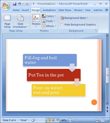
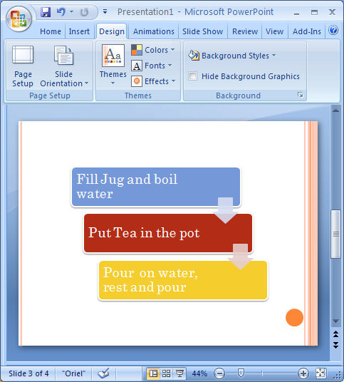
I like the one called Staggered Process which I’ve shown here as it makes a great display for a simple step-by-step process. Select your choice of design and then you’ll see text brackets appear on the screen. Click in them or click the double-pointing arrows at the left of the SmartArt object and type your text in the special dialog.
Once you’ve got your bullet points in – and you can add more than the default three if you need more – you have a simple step-by-step graphic. But – this is only the beginning.
There are lots of different looks for your graphic including beveled edges and 3D effects, and you can choose these from the SmartArt styles dropdown list in front of you. You can also change the colors used in the design which, of course, are based on the current document Theme colors. Change the Design Ttheme and the look of the project changes with it.
It’s about as simple as it’s ever going to be to add great looking step-by-step graphics to a PowerPoint slide. They are, seriously, way cool…
Helen Bradley


Thursday, March 22nd, 2007
Pictures inside Excel comments
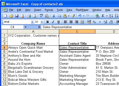
In a previous tip of the day, I showed you how to create shaped comments in Excel but today I’m going to go one step further and create pictures inside the comment.
As you might expect, start off in Excel and add a comment to a cell. Right-click the cell and choose Show comment and then click the border of the comment to select it. Choose Format, Comment and, from the Colors & Lines tab’s Color dropdown list choose Fill Effects and then the Picture tab and click Select Picture.
Find a picture to add to your comment from those in your My Pictures folder, enable the Lock Picture Aspect Ratio checkbox and click OK twice. You’ll now have the image inside your comment.
Depending on the image that you have used you may want to change the format of the text, for example coloring it a different color and sizing it large enough so that it can be easily seen.
For more tips and tricks and helpful Office columns, visit Projectwoman.com
Helen Bradley
Labels: comments, Excel 2003, images
Categories:Uncategorized
posted by Helen Bradley @ 6:27 pmNo Comments links to this post